At Pruna AI, we are huge fans of the FLUX.1[dev] model from the incredible team at Black Forest Lab.

• It’s the highest ranked open-weights model at the Artificial Analysis text-to-image leaderboard.

• With over 8,500 likes, it’s also the most popular model on Hugging Face.

However, due to its 12B parameters, generating a single high-resolution image can take up to 30s on modern hardware - too slow for many applications. Fortunately, there are ways to reduce inference time. In this post, we compare three such approaches: torch.compile, TensorRT, and our own Pruna optimization engine. The summary of this comparison is presented in the table below.

* We measured inference times on an NVIDIA L40S GPU using 50 prompts from NVIDIA’s calibration dataset. The function below calculates the average time needed to generate a single 512×512 image with the default number of inference steps for FLUX.1[dev]:

import time
import torch

def measure_inference_time(pipe)
		# load 50 prompts from NVIDIA's calibration dataset
		with open("calib_prompts.txt", "r", encoding="utf8") as file:
		    prompts = [line.rstrip("\n") for line in file][-50:]
		# measure average time per prompt
		start_time = time.time()
		for prompt in prompts:
		    pipe(prompt, 
		         num_inference_steps=50, 
		         width=512, 
		         height=512,
		         generator=torch.Generator(device="cuda").manual_seed(0)
		         )
		end_time = time.time()
		avg_time = (end_time - start_time) / len(prompts)
		print(f"Average time taken: {avg_time:.2f} seconds")

** The speed up for TensorRT is not reproducible. We followed the official tutorial, but were unable to build a TRT engine. The 2.40x speedup is based on this benchmark from NVIDIA for a different diffusion model running on a different GPU.

How fast is FLUX.1[dev]?

Before diving into the optimization techniques, it’s important to benchmark the FLUX.1[dev] model to establish our starting point. Below is a code snippet that downloads the FLUX.1[dev] model from Hugging Face and measures the average time taken to generate an image.

from diffusers import FluxPipeline

# load FLUX.1[dev] from HuggingFace
pipe = FluxPipeline.from_pretrained(
    "black-forest-labs/FLUX.1-dev",
    torch_dtype=torch.bfloat16
).to("cuda")

# time the FLUX.1[dev] model
measure_inference_time(pipe)

> Average time taken: 8.71 seconds

How fast is FLUX.1[dev] with torch.compile?

Now, let’s see how much we can improve upon the 8.71 seconds per generated image required by the FLUX.1[dev] model. Torch.compile is a can be a reasonable option for model optimization, as it is part of the widely used PyTorch library and only requires one line of code to apply.

When you apply torch.compile to a model such as FLUX.1[dev], it combines TorchDynamo for the execution graph caption and TorchInductor for the backend. Under the hood, it analyzes the forward operations (like matrix multiplications, additions, and activation functions), and determines which operations can be fused or performed with existing Triton kernels to make the forward pass more efficient. This optimization occurs during the first execution of the compiled model, which may take slightly longer than usual. Afterwards, you can expect a 10% to 40% speedup compared to the original model. When compiling the transformer component of the FLUX.1[dev] model which represents the heavy lifting during inference, it would become:

# compile the transformer of the FLUX pipeline
pipe.transformer = torch.compile(pipe.transformer)

# warmup
pipe(eval_prompts[0],
     num_inference_steps=50,
     width=512, 
     height=512
    )

# time the compiled FLUX.1[dev] model
measure_inference_time(pipe)

> Average time taken: 7.08 seconds

Cool! This single line of code provided a 23% speedup over the original model while leaving the generated images unchanged.

How fast is FLUX.1[dev] with TensorRT?

Beyond compilation, several techniques exist that trade off image quality for faster inference. When done correctly, the reduction in quality is negligible, while inference speed can be doubled - or even tripled. One such technique is weight quantization, which is supported by the TensorRT Optimizer.

The idea behind quantization is simple. As mentioned earlier, the FLUX.1[dev] model contains 12B float parameters. Each of the parameters is represented with a limited number of bits. E.g. FLUX.1[dev] uses BFloat16 parameters, meaning each parameter is represented with 16 bits. Quantization aims to reduce the number of bits used per parameter - for example, using 8 bits instead of 16. This has two main benefits: it cuts the memory requirement in half (potentially enabling FLUX.1[dev] to run on smaller GPUs) and, starting with the Ada Lovelace series, NVIDIA GPUs are highly optimized for operations on 8-bit numbers.

Converting from 16 to 8 bits is more challenging than it might seem. A naive approach can significantly degrade model quality, so the conversion must be done intelligently. TensorRT addresses this by offering an enhanced version of SmoothQuant to convert the FLUX.1[dev] model’s BFloat16 parameters into Float8 (FP8) parameters. To use this method, you first need to install the modelopt library via pip.

pip install "nvidia-modelopt[all]" -U --extra-index-url https://pypi.nvidia.com

Running the quantization requires providing several configurations and defining the calibration procedure. While this introduces setup complexity, it also allows you the flexibility to tailor the process to your specific needs. The following code snippet is based on this script from the official TensorRT Optimizer repository.

import modelopt.torch.opt as mto
import modelopt.torch.quantization as mtq

# configuration for quantization
n_steps = 50
width = 512
height = 512
calib_size = 128
format = "fp8"
trt_high_precision_dtype = "BFloat16"
backbone = pipe.transformer

with open("calib_prompts.txt", "r", encoding="utf8") as file:
		calib_prompts = [line.rstrip("\n") for line in file][:128]

def do_calibrate(pipe: FluxPipeline,
                 calibration_prompts: list[str],
                 calib_size: int,
                 n_steps: int, 
                 width: int, 
                 height: int):
    for i_th, prompts in enumerate(calibration_prompts):
        if i_th >= calib_size:
            return
        pipe(prompt=prompts,
             num_inference_steps=n_steps,
             height=height,
             width=width).images

quant_config = {
    "quant_cfg": {
        "*weight_quantizer": {"num_bits": (4, 3), "axis": None},
        "*input_quantizer": {"num_bits": (4, 3), "axis": None},
        "*output_quantizer": {"enable": False},
        "*q_bmm_quantizer": {"num_bits": (4, 3), "axis": None},
        "*k_bmm_quantizer": {"num_bits": (4, 3), "axis": None},
        "*v_bmm_quantizer": {"num_bits": (4, 3), "axis": None},
        "*softmax_quantizer": {
            "num_bits": (4, 3),
            "axis": None,
        },
        "default": {"enable": False},
    },
    "algorithm": "max",
}

for _, p in quant_config["quant_cfg"].items():
    if "num_bits" in p.keys() and "trt_high_precision_dtype" not in p.keys():
        p["trt_high_precision_dtype"] = trt_high_precision_dtype

def forward_loop(backbone):
    pipe.transformer = backbone
    do_calibrate(
        pipe=pipe,
        calibration_prompts=calib_prompts,
        calib_size=calib_size,
        n_steps=n_steps,
        width=width,
        height=height
    )

# quantize backbone
mtq.quantize(backbone, quant_config, forward_loop)

This code snippet took approximately half an hour to run. However, for higher resolution images, the process may take several hours. It is important to understand that quantization alone is not enough to achieve a speed up. In fact, when used directly, the quantized model is slower - in my tests, it took 36 seconds to generate a single image. This is because PyTorch is not optimized for 8-bit operations. To realize the speed gains, you must export the quantized model to ONNX and build a TensorRT (TRT) engine. This is where TensorRT truly excels, as NVIDIA is renowned for optimizing models for its own hardware.

We closely followed this script from the TensorRT repository to export the quantized model to ONNX. It leads to multiple setup obstacles:

• First, even with 64GB of RAM, we encountered out-of-memory errors during the process. We also tried running the quantized model using the DeviceModel interface using the commands provided in this tutorial, but ran into a *torch.onnx.errors.SymbolicValueError* that could not be resolved quickly.

• Next, we launched a new instance equipped with 128GB of memory and set up a Model Optimizer Docker container following the repository’s recommendations. Unfortunately, when running the commands within the container, we received an ImportError from the quantize.py script because it could not import the function convert_float_to_float16 from onnxmltools.utils.float16_converter.

After four hours of troubleshooting, we could not build the TRT engine with reasonable efforts. From experience, setting up and maintaining TRT can take significant time.

Thus, when it comes to the inference speed, we rely on the numbers provided by official TensorRT benchmarks. In this technical blog post, they report a 1.95× speed up over torch.compile using FP8 quantization for a different text-to-image model. Assuming a similar improvement for FLUX.1[dev], this would reduce the image generation time to approximately 3.63 seconds per image - a 2.4× speed up over the original version. As mentioned earlier, this speed up comes with a slight loss in performance. We will revisit this aspect at the end of the blog post.

How fast is FLUX.1[dev] with Pruna?

Beyond quantization, we can also use a technique called caching, which reuses the output of previous diffusion steps to avoid expensive computations. The Pruna package offers a flux_caching method with two parameters. Typically, it is not advisable to use caching during the first few steps, so the start_step parameter determines the inference step at which caching begins, while the cache_interval parameter specifies for how many steps the cached output is reused.

After installing Pruna with

pip install pruna[gpu]==0.1.2 --extra-index-url https://prunaai.pythonanywhere.com

you can simply run flux_caching with less than 10 lines of code:

from pruna import SmashConfig, smash

# your token (you get it when running smash for the first time)
token = <your_token>

smash_config = SmashConfig()

# configure the caching
smash_config["cachers"] = ["flux_caching"]
smash_config["cache_flux_caching_start_step"] = 5
smash_config["cache_flux_caching_cache_interval"] = 3

smashed_pipe = smash(model=pipe,
					token=token, 
					smash_config=smash_config)

# time the smashed model
measure_inference_time(smashed_pipe)

> Average time taken: 3.82 seconds

While it provides already good speed up, you can do better by combining it with compilation. The great thing about the Pruna package is that you can easily stack different techniques. In the following snippet, we add the diffusers2 compiler on top of flux_caching with just one additional line of code.

smash_config = SmashConfig()

# configure the caching
smash_config["cachers"] = ["flux_caching"]
smash_config["cache_flux_caching_start_step"] = 5
smash_config["cache_flux_caching_cache_interval"] = 3
# configure the compilation
smash_config["compilers"] = ["diffusers2"]

# warmup
smashed_pipe = smash(model=pipe,
					token=token, 
					smash_config=smash_config)
										 
# time the smashed model
measure_inference_time(smashed_pipe)

> Average time taken: 3.24 seconds

In summary, by combining flux_caching with diffusers2, we achieved a 2.7× speed up compared to the original model. We can push performance even further by e.g. using LoRA adapters, or incorporating techniques such as Hyper-SD, which enable faster generation of high-quality images with fewer inference steps - but that may be the subject of another blog post.

The results for our inference time measurements are summarized in the plot below.

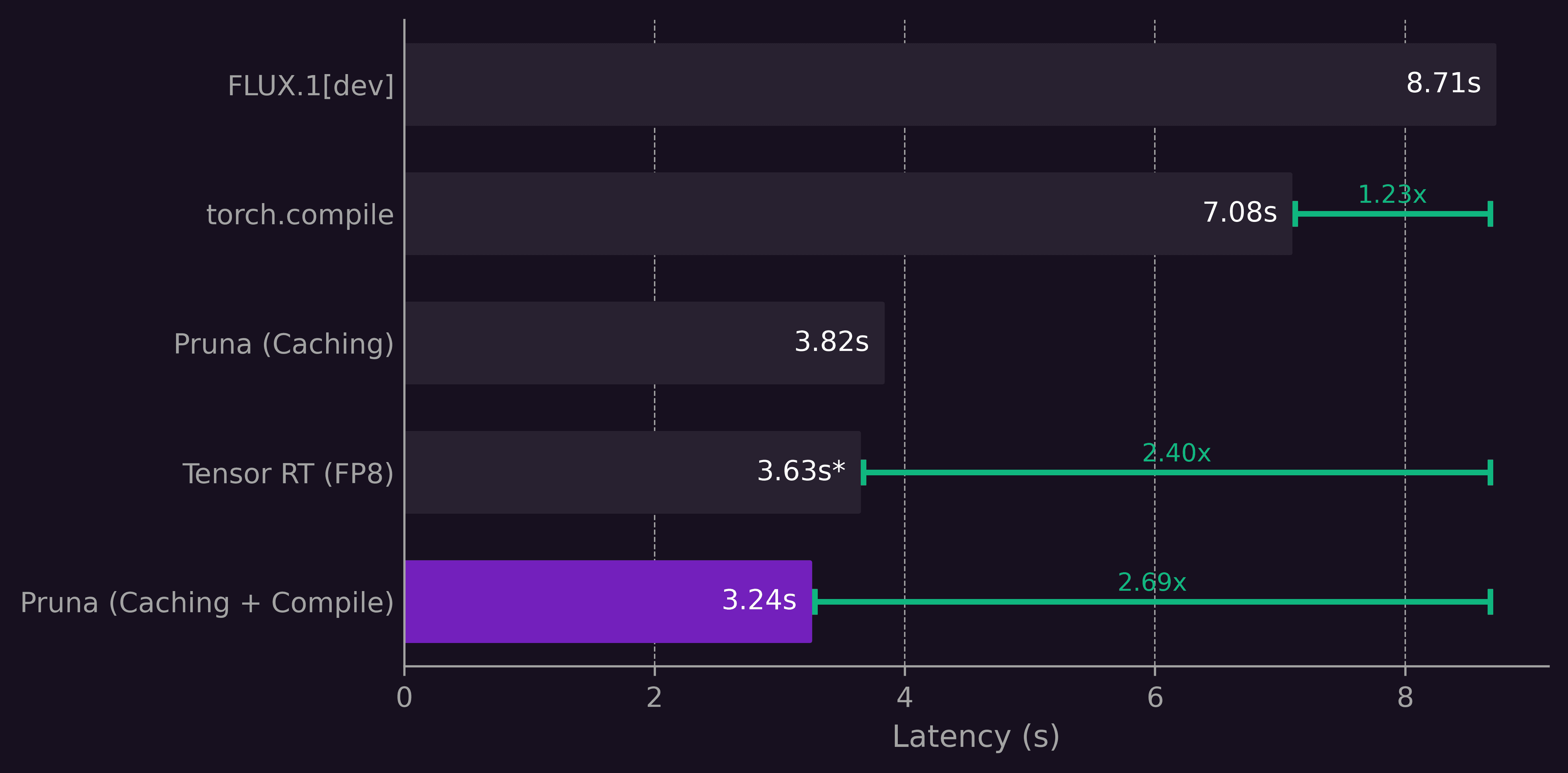
The speed-up for TensorRT is not reproducible. We followed the official tutorial, but were unable to build a TRT engine. The 2.40x speedup is based on this benchmark from NVIDIA for a different diffusion model running on a different GPU.

Evaluating Image Quality

To evaluate image quality, we compared the images generated by the base model with those produced by the compressed models. Specifically, we computed LPIPS, SSIM, and PSNR - metrics commonly used in scientific literature. While these scores provide useful insights, it is worth noting that an image can exhibit higher quality even if it differs from the original. The table below presents the average scores for both the TensorRT and Pruna models across 50 evaluation prompts.

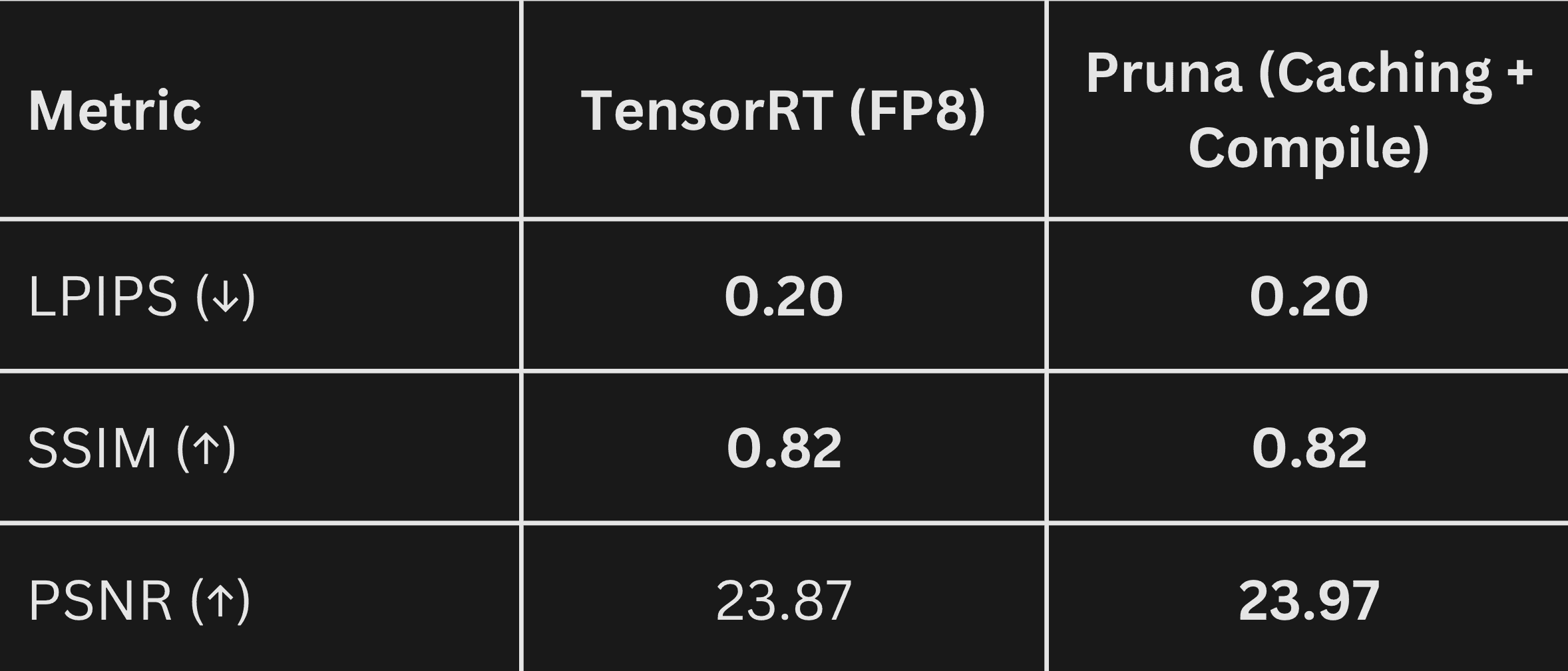
While the Pruna model is faster, it performs comparably according to these metrics compared to the TensorRT model. Since numbers alone can’t capture the full picture, we’ve also included side-by-side comparisons of the generated images to provide a better visual understanding.

It’s remarkable that, despite the reduced generation time, the images produced by the quantized and cached model so closely match those of the original. This really showcases the huge potential of efficient machine learning techniques to FLUX.1[dev].

Conclusion

Generating images with FLUX.1[dev] doesn’t have to be slow. Using torch.compile is straightforward and offers a 1.23× speedup. TensorRT’s model quantization cuts latency further but can be hard to set up and requires time for calibration. With the Pruna package, we address these challenges by prioritizing user experience. Our flux_caching method takes fewer than ten lines of code and needs no calibration. Combined with compilation, it delivers a 2.69× speedup while matching TensorRT’s image quality. Looking ahead, we plan to publish quantization methods for FLUX.1[dev] as well. Ideally, we could combine quantization, caching, and compilation to achieve even greater speedups. Stay tuned!